Cycle Time Calculation for Better Efficiency

At its core, the simplest way to figure out your cycle time is to divide your Net Production Time by the Number of Units Produced. This gives you a raw, unfiltered look at your process speed—how long it really takes to get one unit of work done from the moment you start until it’s finished.

The Core Formula Explained

Cycle time is a fundamental metric that tells you the total time it takes to produce a single item, warts and all. It includes the productive work and all the little non-productive moments in between, making it a powerful gauge of your team’s real-world efficiency. If you want a more detailed breakdown, we have a complete guide on the cycle time definition.

Let’s make this tangible. Say your team works an 8-hour shift, but you lose 3 hours to meetings and other interruptions. That leaves you with a net production time of 5 hours. If the team completes 200 units in that time, your cycle time is a straightforward 1.5 minutes per unit. This simple number is your first clue to benchmarking efficiency and finding where things are getting stuck.

The real power of calculating cycle time isn’t just in the final number. It’s in understanding what “net production time” actually contains. This isn’t just coding time; it includes PR reviews, QA, waiting for deployment, and all the small delays that add up.

To get the most out of this metric, it helps to break down the formula into its core components.

Cycle Time Formula Components

Component	Definition	Example Value
Net Production Time	The total available time for work after subtracting all planned and unplanned downtime (e.g., meetings, breaks).	5 hours (8-hour day - 3 hours downtime)
Number of Units	The total count of completed work items (e.g., features, tickets, bug fixes) within that production time.	200 units
Cycle Time	The average time it takes to produce one single unit of work.	1.5 minutes

This table clarifies how each element contributes to the final calculation, giving you a clear picture of where to focus your improvement efforts.

Average Vs. Ideal Cycle Time

It’s also crucial to know the difference between the cycle time you have and the one you want.

• Average Cycle Time: This is your reality. It’s the metric that includes all the real-world delays, interruptions, and context switching that happen on any given day. It’s what you’re actually achieving.
• Ideal Cycle Time: This is your best-case scenario. It’s the theoretical minimum time needed to complete a task if everything went perfectly, with zero interruptions. Think of it as your performance benchmark.

Getting a handle on your cycle time is one of the most direct ways to improve throughput and reduce costs. For instance, quality inspection and code review time are often a surprisingly large part of the equation, sometimes eating up 5-15% of the total cycle time, depending on how complex the work is. By tracking both your average and ideal times, you can start to see just how much room there is for improvement.

Getting More from Your Cycle Time Metric

Cycle time is more than just a number on a dashboard; it’s a direct reflection of your team’s rhythm and its ability to keep pace with what customers actually want. The real magic happens when you start comparing your cycle time to your takt time.

Think of takt time as the pulse of customer demand. It’s the rate you need to produce at to meet your commitments. You calculate it by dividing your available production time by the required output. Once you have that number, your cycle time suddenly goes from a simple metric to a powerful gauge of your team’s true performance.

What Takt Time Tells You

Comparing these two numbers gives you immediate, actionable insights.

• Spotting Idle Capacity: If your cycle time is consistently lower than your takt time, you’ve got slack in the system. This isn’t necessarily a bad thing, but it’s an opportunity to rebalance work or pull in more tasks without overwhelming the team.
• Seeing Capacity Risks: When cycle time starts creeping up past your takt time, alarm bells should go off. You’re now at risk of falling behind, missing delivery targets, and frustrating your users.
• Finding Your Focus: The gap between the two metrics points you directly to your most impactful improvement projects. Instead of guessing where to optimize, you know exactly where the friction is.

By viewing cycle time through the lens of market demand, it becomes a key strategic indicator. Imagine a team working two 8-hour shifts (960 minutes) needs to ship 160 units of work. Their takt time is 6 minutes per unit. If their actual cycle time is only 3 minutes, they have extra capacity. But if it stretches beyond 6 minutes, they’re going to miss their targets. You can read more about the relationship between cycle and takt time on Tulip.co.

Calculating the Real Cost of Slowdowns

So, how do you put a number on this? You can quantify cycle time losses by taking your actual run time, subtracting the ideal cycle time, and then multiplying that by the number of units produced. It’s not uncommon for teams to discover that these losses eat up 20–25% of their productive time before they start digging in and making improvements.

Measuring these losses isn’t about pointing fingers; it’s about pinpointing exactly where to focus your efforts to eliminate waste and streamline your process.

Turning Metrics into Action

Getting these numbers right depends on solid instrumentation. Modern analytics stacks make it possible to track work as it happens. We see teams across the globe using these insights to fine-tune their planning and slash lead times.

For example, a common setup involves developers using tools like Zest plugins or simple event tagging in VS Code, then streaming that data into dashboards in Grafana or Power BI. This gives them the ability to:

1. Allocate work based on real-time throughput, not guesswork.
2. Get alerts on bottlenecks before they derail a sprint.
3. Spot quality issues earlier by flagging deviations from the norm.
4. Balance team workloads to keep everyone engaged and productive.

Dashboards are great for spotting trends, helping you predict and prevent future cycle time blowouts before they even happen.

Your Next Improvement Steps

Once you can see where the time is going, you can start running targeted experiments to tighten things up. You don’t have to boil the ocean. Start small with a pilot project or use AI-assisted coding sessions in Zest to quickly validate a hunch about a process change.

Here are a few practical ideas to get you started:

• Try smoothing out the workload by rotating complex tasks across the team.
• Run a quick Kaizen event focused solely on the single biggest time sink you’ve identified.
• Dig into AI Metrics from Zest sessions to find recurring patterns of slowdowns.
• Set up simple, automated alerts that fire whenever your cycle time exceeds your takt time.

Make sure you review the results of these experiments with your team and other stakeholders, and be ready to adapt. This whole process is about iterative testing and creating tight feedback loops—that’s the real heart of lean improvement.

Ultimately, aligning your cycle time with customer demand (takt time) empowers your team to work at a sustainable, predictable pace.

• Use visual dashboards and daily standups to help the team own their metrics and sustain improvements.
• Lean on AI Hints in Zest to get an early warning when cycle time starts to drift.

By constantly monitoring your cycle time against takt time and tracking your losses, you’ll know exactly where to invest your improvement efforts to get the biggest bang for your buck.

How to Reliably Collect Cycle Time Data

Your cycle time calculation is only as good as the data you feed it. If you’re still relying on manual stopwatches or cobbled-together spreadsheets, you’re not getting a clear picture. Those methods are full of errors and just can’t keep up with the complexity of modern software development.

To get insights you can actually trust, you need to automate your data collection. The idea is to have it all happen in the background, logging timestamps and events without anyone having to think about it. This way, you get a record of what really happened, not just what people remember.

Modern Instrumentation Techniques

It’s time to ditch the tedious manual tracking. Today’s tools let you pull data directly from the source, and for engineering teams, that means integrating collection right into the development environment.

• AI-Assisted Recording: Tools like Zest offer plugins that automatically log start and end times for tasks during an AI-assisted coding session. This captures super granular data on how long specific sub-tasks take without developers lifting a finger.
• IDE Event Tagging: With a simple VS Code extension, a developer can tag key moments—like start_coding, pr_submitted, or review_started—with a quick command. This creates a clean, structured event log that’s worlds more reliable than trying to reconstruct a timeline from Git commit history.
• Manufacturing Sensors: Stepping outside of software for a moment, think about a factory floor. IoT sensors can automatically timestamp when a part enters and leaves a station. This provides a precise, undeniable log for every single stage.

When you build data collection into the daily workflow like this, you end up with a rich, trustworthy dataset—the perfect foundation for accurate cycle time analysis.

Setting Up Your Data Pipeline

Capturing the events is just the first step. You need a central hub to store and process all that information. A solid data pipeline is what turns raw data into clean, synchronized, and visualization-ready insights.

A popular and effective approach is to stream event data from your sources—whether it’s VS Code or a factory sensor—into a time-series database.

Pro-Tip: Don’t let your data pipeline be a passive bucket. It should actively clean and structure the data as it comes in. For example, it can automatically link a pr_merged event back to its corresponding start_coding event, giving you a complete, end-to-end record for that piece of work.

Tools like Elasticsearch or InfluxDB are fantastic for this. They’re built to handle massive volumes of timestamped data and make it easy to query for specific events or time ranges. This setup gets your data prepped for dashboards and further analysis. If you’re looking for a more all-in-one solution, exploring different developer time tracking software options can uncover tools that handle both capture and analysis seamlessly.

This infographic shows how cycle time fits into the bigger picture of meeting customer demand, which is represented by takt time.

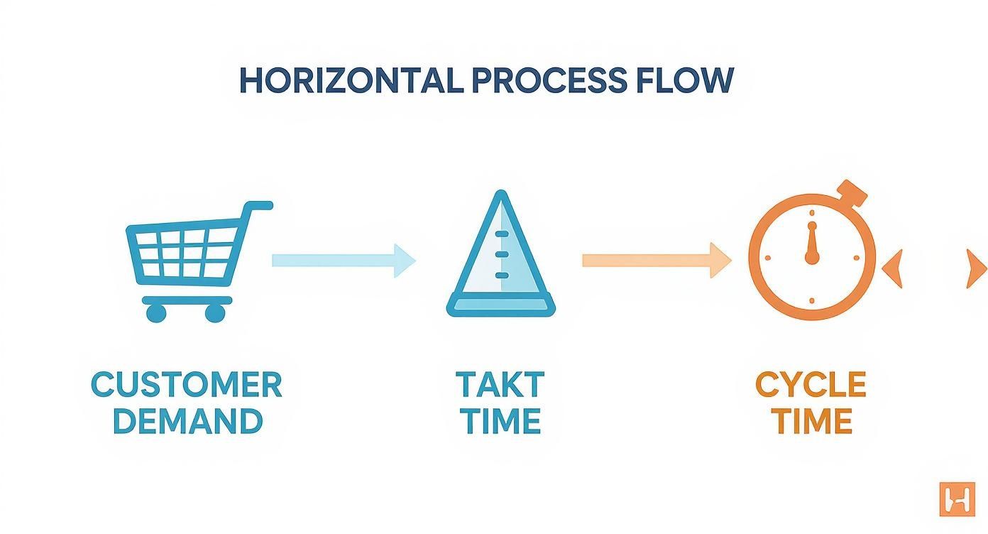
As you can see, takt time is the pace you need to maintain to keep up with demand, while cycle time is the pace you’re actually hitting. The difference between the two is a direct measure of your team’s operational efficiency.

Cleaning Your Data for Accurate Insights

Let’s be honest, raw data is messy. A single production fire that pulls everyone off their tasks, a bug that turns into a multi-day spelunking expedition, or even just a ticket updated incorrectly can throw your cycle time metrics way off.

These extreme outliers are the data equivalent of a 10-car pileup on the freeway. If you included that one terrible commute in your daily average, it would completely misrepresent your typical drive time. The same thing happens here. Ignoring these anomalies will give you a skewed, inaccurate picture of your team’s actual performance.

To get a real feel for your delivery pace, you have to handle these exceptions thoughtfully.

Identifying and Handling Outliers

The goal here isn’t to cherry-pick the data to make your team look good. It’s about systematically filtering out the genuine statistical noise so you can see the real signal underneath. This ensures the metrics you share are both accurate and defensible.

A couple of statistical methods work really well for this:

• Interquartile Range (IQR): This is my go-to when the data is a bit wild and doesn’t follow a neat bell curve. It works by focusing on the middle 50% of your data, so it isn’t easily fooled by a few ridiculously long or short cycle times. You essentially find the range between the 25th percentile (Q1) and the 75th percentile (Q3) and flag anything that falls too far outside that box.

• Z-Score Thresholds: This approach is perfect if your cycle time data is more predictable and clusters around an average. It measures how far each data point is from the mean, in terms of standard deviations. A common rule of thumb is to flag anything with a Z-score greater than 3 as an outlier.

The most important thing is to decide on your rules before you start cleaning and to write them down. For example, you might create a policy to filter out any task that takes more than three standard deviations from the mean. This keeps the process consistent and unbiased.

Setting Sensible Filtering Limits

So, which method should you choose? If your cycle times are all over the map, with a few tasks taking weeks while most take days, the IQR method is probably your safest bet. If your data is more clustered, Z-scores are a clean and effective way to go.

Whatever you decide, document it. When you show your cycle time charts to stakeholders, you need to be able to explain precisely what you filtered out and why. This transparency is crucial for building trust in your numbers.

For example, a team might agree on a simple, clear rule: “For our weekly reporting, we exclude any ticket with a cycle time above the 95th percentile from the last quarter.” This removes the extreme, one-off delays from your average without completely ignoring them—you can always analyze those edge cases separately to find bigger process issues.

By taking the time to clean your data, your cycle time calculation transforms from a noisy guess into a reliable indicator of your team’s typical throughput. It becomes a solid foundation for making much smarter decisions.

Making Cycle Time Metrics Visible And Actionable

You can clean your data endlessly, but if cycle time lives in a spreadsheet no one checks, it won’t spark progress. Pinning those numbers to a live dashboard turns them into a shared story that engineers and executives can rally around.

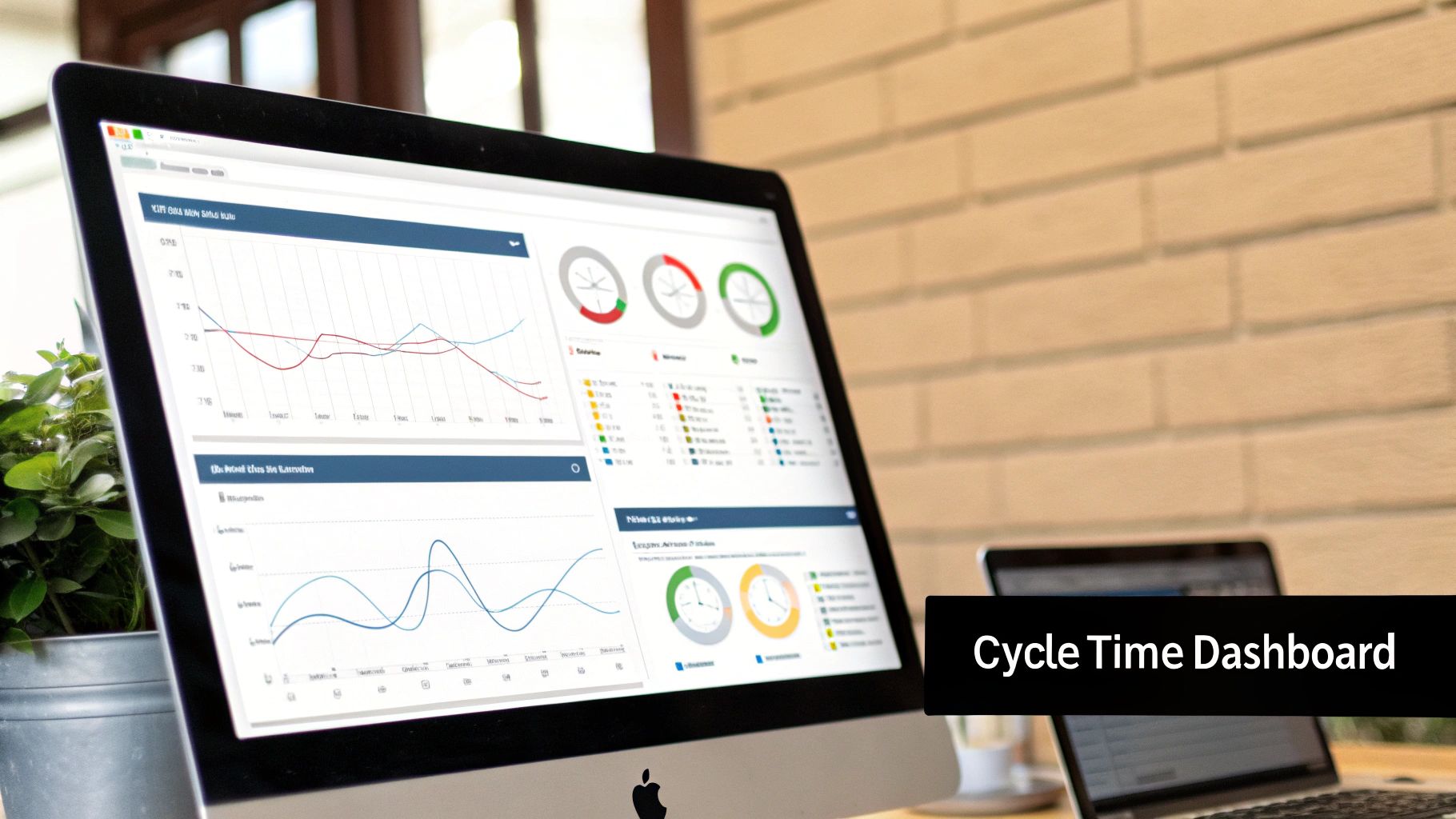
The real power of visualization isn’t in pretty colors—it’s in surfacing trends, bottlenecks, and quick wins. Swap out static slides for an interactive view that highlights exactly where your team’s time is going.

Designing Dashboards That Drive Decisions

A smart dashboard answers critical questions before you ask them. Instead of displaying only the current average cycle time, it uncovers the deeper rhythms of your workflow.

• Time-Series Charts — Plot average cycle time over days, weeks, or months to identify upward or downward trends.
• Control Charts — Add upper and lower control limits to your cycle time points. Any dot outside those bounds is an instant red flag.
• Heat Maps — Visualize each stage (coding, review, testing, deployment) so “hot” cells pinpoint the biggest delays.

When you show that a 10% cut in code review time boosts feature throughput by 5%, alignment and funding happen almost automatically.

From Visualization To Automation

Today’s BI platforms make this setup a breeze. With a few clicks, you can connect to sources like Elasticsearch or InfluxDB and drag your charts into place. Consider tools like Grafana or Power BI for seamless data pulls and real-time dashboards.

You can even automate alerts. For instance, configure Grafana to send a Slack message when the 24-hour average cycle time exceeds your target. That way, your team gets a heads-up immediately instead of waiting for a weekly summary.

Many teams pair cycle time with what DORA metrics are to round out their delivery picture.

Manufacturing research underscores how valuable this is. Lean factories zeroing in on cycle time often see 20-30% productivity gains. In one case, a line slashed its unit time from 90 to 60 seconds—a 33% boost in throughput and a sharp drop in costs.

Discover these manufacturing improvements on mrpeasy.com for more real-world examples.

Putting Your Tools into Practice

https://www.youtube.com/embed/cSRblWIiC4Q

Alright, let’s move from theory to reality. Getting a live monitoring system up and running is where you’ll see the real power of cycle time. The idea isn’t just to collect data; it’s to embed measurement right into your team’s daily workflow without getting in their way. This is where the tools you already use, like VS Code, can become incredibly powerful when paired with specialized plugins like Zest.

A solid setup begins right where the work happens: the IDE. Instead of asking developers to manually log their time, you can create a super-lightweight event-tagging system inside VS Code. It could be as simple as a few custom snippets or a small extension that lets a developer tag key moments—task:start, review:begin, merge:complete—with a quick command. This creates a clean, structured stream of data that becomes the foundation for all your calculations.

Integrating Zest for Deeper Insights

While manual tagging is a good first step, tools like Zest can automate nearly the entire process. When you use Zest for AI-assisted coding sessions, it automatically logs the start and end times for tasks and even smaller sub-tasks. You get a granular, moment-by-moment picture of the development process without anyone having to lift a finger.

This automated data capture is a goldmine for writing simple, maintainable plugin scripts. For instance, you can write a quick script that listens for Zest events and pushes them directly to your analytics endpoint.

Here’s a quick look at what that might conceptually look like:

// Zest Plugin Script Example zest.on(‘session.end’, (sessionData) => { const cycleTimeData = { taskId: sessionData.taskId, startTime: sessionData.startTime, endTime: sessionData.endTime, durationMs: sessionData.duration, };

// Push to your analytics platform sendToGrafana(cycleTimeData); });

This kind of setup ensures your data is not only accurate but also consistently captured, giving you a rock-solid foundation for your dashboards.

Piping Data into Analytics Platforms

Once you’re capturing events from VS Code and Zest, the next move is to send that data to an analytics platform like Grafana. This is where your raw event logs get transformed into meaningful visualizations. You can set up a data pipeline that feeds a time-series database—something like InfluxDB or Elasticsearch works great and plays nicely with Grafana.

Inside your Grafana dashboard, you can then build queries that calculate the time between different event tags. For example, a query could measure the duration between review:begin and merge:complete to give you a precise “Code Review Time.”

A critical part of making this work is automating data validation. Set up simple checks in your pipeline to flag incomplete records, like a task:start event that never got a corresponding task:end. This keeps your dataset clean and your metrics trustworthy.

You can even use simple AI prompts with a tool like ChatGPT to spot anomalies in your raw data before it ever hits your dashboards. Just feed it a chunk of event data and ask, “Identify any cycle times that are statistical outliers based on the 95th percentile.” This can quickly flag issues that need a closer look, helping you maintain data quality without bogging down your team.

Answering the Tough Questions About Cycle Time

Even when you’ve got the formula down, putting cycle time tracking into practice always brings up a few tricky questions. I’ve seen teams get stuck on these details time and again, so let’s clear up the most common points of confusion.

Should I Use an Average or an “Ideal” Cycle Time?

This one trips up a lot of people, but the answer is simple: you need both, but for different reasons.

Average cycle time is your reality. It’s the unfiltered truth of how long things actually take, including all the messy interruptions, unexpected delays, and context switching. This is the number you should use for reporting on past performance and for realistic capacity planning. It’s what is.

Ideal cycle time, on the other hand, is your north star. Think of it as the “perfect run”—the absolute fastest a task could get done if everything went right. This isn’t for reporting; it’s a benchmark for improvement. When you make a process change, you can measure how much closer it gets you to this ideal. It’s what could be.

How Do I Know What Data to Filter Out?

Filtering outliers is a balancing act. You want to remove genuine one-off anomalies that would throw off your average, but you don’t want to hide real, recurring problems. It’s easy to massage the numbers to look good, but that defeats the whole purpose.

A solid, statistically-sound approach is to exclude anything that falls above the 95th percentile. This reliably cuts out the extreme edge cases—that one ticket that got stuck in review for a month—without masking systemic friction.

Whatever you decide, write it down and make it public. Transparency is everything when it comes to metrics. A simple, clear policy like, “We filter out any task that takes more than 3x our quarterly average cycle time,” builds trust and keeps everyone on the same page.

Wait, What’s the Difference Between Cycle Time, Lead Time, and Takt Time?

It’s easy to get these mixed up, but they measure distinct parts of your workflow. Getting them straight is key to seeing the full picture.

• Cycle Time: This is your internal clock. It measures how long it takes your team to complete a piece of work from the moment they start coding to the moment it’s done. It’s all about your internal process efficiency.

• Lead Time: This is the customer’s clock. It starts ticking the second the customer makes a request and doesn’t stop until that request is delivered. This is the total wait time they experience.

• Takt Time: This is the market’s clock. It’s not about how fast you are, but how fast you need to be to keep up with customer demand. You calculate it based on demand, not your team’s current speed.

Ready to stop guessing and start measuring your team’s true development rhythm? Zest integrates directly into your AI coding workflow, automatically capturing the data you need to calculate cycle time accurately. Spot bottlenecks, share best practices, and drive real improvement. Get started with Zest for free.

---

Master Your Cycle Time Calculations

Turn raw process data into a clear, actionable metric for improving delivery speed and predictability.

📊 Core Metrics

1. Average Cycle Time — The real-world time from task start to completion.
2. Ideal Cycle Time — Your theoretical best-case scenario for a single task.
3. Outlier Percentage — The percentage of tasks filtered out based on your rules.

🕹️ My Cheatcodes

• 🌱 Distinguish Your Times — Use 'Average' for reporting what happened and 'Ideal' for setting improvement goals.
• 🦎 Filter with Rules — Set a clear, documented policy (like the 95th percentile) for removing outliers consistently.
• ⚡ Know Your Times — Remember: Cycle Time is your process speed, Lead Time is the customer's wait, and Takt Time is the market's demand.

📈 Reflection Points

• 💡 Is my current 'average' cycle time hiding systemic delays we've just accepted as normal?
• 🧩 Are we filtering outliers to get an accurate picture or just to make the numbers look better?
• 📘 Does my team understand the difference between cycle, lead, and takt time?