Calculating Cycle Times for Software Teams

Calculating cycle time is all about measuring the total time that passes from when work actively begins on an item until it’s finished. Think of it as your team’s internal clock—it reveals the true speed of your development process. Nailing this down is one of the most powerful things you can do to improve predictability and shine a light on hidden inefficiencies.

What Is Cycle Time and Why Should You Care

At its heart, cycle time is one of the most honest metrics you can track. It’s not about how busy people look; it’s about how quickly real work actually flows through your system.

Let’s use a simple analogy. Imagine you’re ordering a custom-built desk. The cycle time doesn’t start when you place the order. It starts the moment a carpenter picks up the first piece of wood and begins working. It ends when the desk is fully assembled and ready to be shipped. That’s it. That’s the work time.

This simple concept is a game-changer for a few key reasons:

• It brings predictability to your planning. When you have a solid grasp of your average cycle time, you can give stakeholders realistic delivery forecasts instead of just guessing. That builds trust and makes sprint planning far more accurate.
• It exposes the real bottlenecks. Are pull requests sitting stagnant for days? Is there a long, painful handoff to the QA team? Consistently high or wildly fluctuating cycle times are a huge red flag, pointing you directly to the friction in your workflow.
• It fuels genuine, continuous improvement. You can’t fix what you can’t see. By tracking cycle time, your team can measure the actual impact of any process changes you make, creating a data-driven culture of efficiency. It’s a cornerstone for high-performing teams and a key part of frameworks like the DORA metrics.

Clearing Up Common Confusion

It’s really common for people to mix up “cycle time” with “lead time” and “takt time.” They sound similar, but they answer very different questions about your process. This isn’t just a software thing; these terms come from the world of manufacturing, where getting them right is crucial for hitting production targets.

Let’s finally put this confusion to rest. Here’s a quick comparison to help you keep them straight.

Cycle Time vs Lead Time vs Takt Time

A quick comparison of the three key time-based metrics in development and operations.

Metric	Starts When	Ends When	Primary Question Answered
Cycle Time	Work actively begins on a task.	The task is completed and ready for the next step.	How long does it take us to do the work?
Lead Time	A request is made by a customer or stakeholder.	The request is delivered to the customer.	How long did our customer wait?
Takt Time	N/A (It’s a calculated rate)	N/A (It’s a calculated rate)	How fast do we need to work to meet demand?

Getting this distinction right is the first real step. Once you’re clear on what you’re measuring, you can start calculating cycle times effectively and using them to make meaningful improvements to how your team builds software.

Mapping Your Workflow for Accurate Measurement

Before you can even think about calculating cycle times, you need a crystal-clear picture of the process you’re actually measuring. We’ve all heard the old saying, “you can’t improve what you don’t measure,” but I’d add a crucial amendment: you can’t measure what you haven’t clearly defined.

Those generic “To Do,” “In Progress,” and “Done” columns on a Jira or Linear board? They’re a decent starting point, but they hide all the juicy details—the bottlenecks, the wait states, the real story of how work gets done.

To get data that actually means something, you have to map the real-world journey a task takes from the moment a developer types the first line of code until it’s live. This means shattering that vague “In Progress” blob into the distinct, granular steps that reflect how your team really operates.

The whole point of this exercise is to nail down the unambiguous start and end points for your cycle time. Everyone on the team needs to be on the same page with this definition. If they aren’t, you might as well be measuring with a rubber band—your data will be totally unreliable.

What Are Your Real Workflow States?

So, what does this look like in the wild? A typical software development workflow is much more nuanced than just “doing the work.” It often includes stages like these:

• Ready for Dev: The ticket is groomed, prioritized, and just waiting for an engineer to grab it.
• Coding in Progress: This is active keyboard time. Someone is writing code.
• Awaiting Code Review: The code is done, but it’s sitting in a queue. This is a classic “wait state” and, from my experience, one of the most common places for work to get stuck.
• In QA: The feature is now being actively poked and prodded by a quality assurance team or running through automated test suites.
• Ready for Deployment: It passed! The work is staged and just waiting for the next release train to leave the station.

Make it Your Own

The states you choose must reflect your team’s unique process. Does your team have a dedicated QA department? Then you absolutely need an “In QA” state. If your developers are responsible for their own testing, maybe that work just gets absorbed into “Coding in Progress.” There’s no right or wrong answer, only what’s true for you.

Here’s the bottom line: Your goal is to create a workflow map that is an honest reflection of your reality. Don’t map the process you wish you had; map the process you actually have. This is the only path to getting data that uncovers real opportunities for improvement.

Once you’ve got this map laid out, you can finally make the big decision: what officially starts and stops the clock for your cycle time? For many engineering teams, the clock starts ticking when a ticket moves into “Coding in Progress” and stops when it hits “Ready for Deployment.”

Whatever you decide, write it down, share it, and stick to it. This consistent definition is the bedrock of everything that comes next.

How to Actually Calculate Your Cycle Time

Alright, you’ve mapped out your workflow. Now for the fun part: the math. Don’t worry, calculating cycle time isn’t as complicated as it sounds. The basic formula is surprisingly simple, and it’s the starting point for all the really insightful analysis.

At the end of the day, it all boils down to this:

End Date - Start Date = Cycle Time

That’s really it. For any single task, you just take the timestamp when it was officially “Done” and subtract the timestamp when work “Started.” The difference is your cycle time for that one piece of work.

A Quick Jira Example

Let’s make this real with a typical Jira ticket.

Say your ticket, DEV-123, has the following history:

• Moved to “Coding in Progress”: 2023-10-23 at 09:00 AM
• Moved to “Ready for Deployment”: 2023-10-25 at 05:00 PM

Plugging that into our formula: Oct 25, 5:00 PM - Oct 23, 9:00 AM = 2 days and 8 hours

Easy enough, right? This gives us the cycle time for a single ticket. But a single data point doesn’t tell you much—it’s just a number without context. To truly understand your team’s delivery rhythm, you need to look at these times in aggregate.

Why Averages Aren’t Enough

The first impulse for most teams is to just calculate the average cycle time. You add up all the individual times over a sprint or a quarter and divide. It’s a decent first step, but averages can be incredibly misleading. All it takes is one or two massive outliers—those tasks that got stuck for weeks—to skew the number and make your team look much slower than it actually is.

This is where percentiles come in. They paint a much more accurate and useful picture of your team’s consistency and predictability.

Percentiles reveal your team’s reliability. Instead of one skewed number, you get a realistic range. Knowing that 85% of your work is completed in 5 days or less is a much more powerful and defensible forecast than saying your “average” is 4 days.

Here are the percentiles I always recommend tracking:

• 50th Percentile (Median): This is your typical case. Half of your work gets done in this amount of time or less.
• 85th Percentile: I consider this your reliability benchmark. You can confidently promise stakeholders that 85 out of 100 tasks will be finished within this timeframe.
• 95th Percentile: This number shines a light on your worst-case scenarios. It helps you quickly spot the outliers that need a closer look.

What About Weekends and Holidays?

This question comes up all the time. Should you count non-working days? The answer depends on your goal.

If you’re trying to diagnose your internal process efficiency—how fast the team moves when they are actively working—then excluding weekends makes sense.

But for everything else, especially predictability and communicating with stakeholders, always use calendar days. Your customer doesn’t really care that a delay happened over a three-day weekend; they just know their feature took longer to arrive.

While the core concept is simple, things can get tricky in the real world when you factor in things like system downtime or other blockers. This complexity is why cycle time is often debated, with different organizations measuring it in slightly different ways.

Ultimately, shifting your focus from simple averages to percentiles will give you a far more robust and honest view of your team’s performance. It moves you from guesswork to making genuinely predictive statements. This data is also a crucial input for other key metrics, as you can see in our guide on how to measure velocity.

Bringing Your Cycle Time Data to Life

Let’s be honest: raw numbers in a spreadsheet rarely spark change. The real magic happens when you turn that data into a visual story your whole team can grasp in a few seconds. Visualizing your cycle times transforms abstract timestamps into clear, undeniable signals about your workflow’s health, shining a light on hidden bottlenecks and celebrating genuine progress.

So, how do you get started? First, you’ll need to pull the raw timestamp data from your project management tool. Most platforms like Jira have powerful query languages to help you pinpoint exactly what you need. A simple Jira Query Language (JQL) query to find all tasks completed last quarter might look something like this:

project = "YourProject" AND status = "Done" AND resolutiondate >= startOfQuarter()

Once you’ve exported this data, you’re ready to build charts that illuminate your team’s real delivery patterns. While you can slice and dice the data in countless ways, a couple of specific charts are absolute game-changers for understanding cycle time.

The Cycle Time Scatter Plot

If you want to spot outliers and get a feel for the consistency of your workflow, the scatter plot is your best friend. Each dot on this chart represents a single completed task, plotted by its completion date (horizontal axis) and its cycle time (vertical axis).

It’s surprisingly easy to read once you know what to look for:

• Tight Clusters: A dense group of dots near the bottom of the chart is exactly what you want to see. It’s a clear sign that most of your work gets done quickly and predictably.
• Outlier Dots: See those dots floating high above the main cluster? Those represent tasks that took way longer than average. These are your red flags, the perfect candidates for a retrospective to figure out what went sideways.
• Drifting Trends: Keep an eye on the overall pattern over time. Is the entire cluster of dots slowly creeping upward? That’s a signal that your cycle time is increasing, hinting at a systemic issue that needs attention.

This scatter plot is a great example—you can immediately see which work items are the outliers and get a sense of the overall distribution.

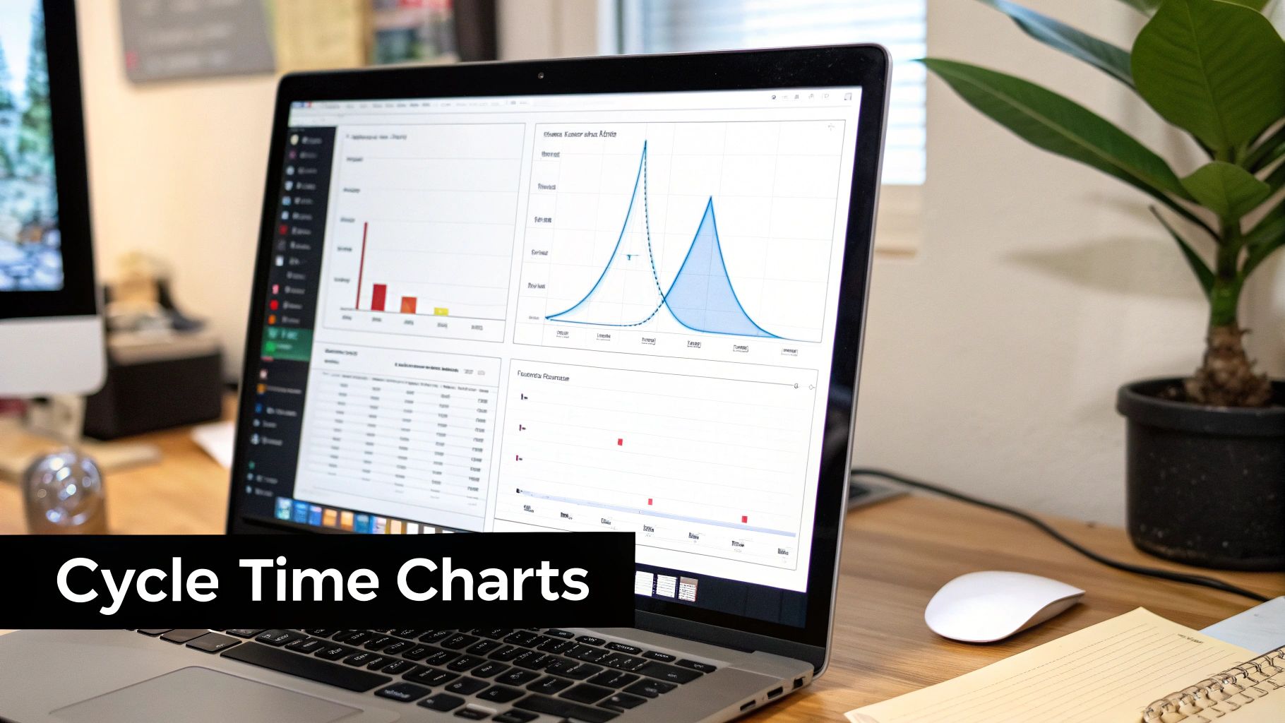
A chart like this gives you so much more context than a simple average ever could.

The Cycle Time Histogram

While a scatter plot gives you the story of individual items, a histogram tells the story of your system as a whole. It groups completed tasks into time-based buckets (like 0-2 days, 3-5 days, 6-8 days) and shows you how many tasks fall into each one.

A histogram moves the conversation away from individual outliers and toward overall system performance. It helps answer the crucial question: “How long does work usually take around here?”

A healthy histogram has a tall bar on the left with a long, tapering “tail” stretching out to the right. This shape tells you that the vast majority of your work finishes quickly, with only a few items taking longer. If you see multiple peaks or a wide, flat distribution, it’s a sign that your process is unpredictable and chaotic.

For a deeper look at related metrics, you might want to check out our guide on key engineering performance indicators.

Common Cycle Time Visualization Methods

To summarize, different charts tell different parts of the story. Here’s a quick breakdown of the most common visualization methods and what they’re best at revealing.

Chart Type	What It Shows	Best For Identifying
Scatter Plot	Each individual work item’s cycle time over a period.	Outliers, trends over time, and process consistency.
Histogram	The frequency distribution of cycle times across time buckets.	The predictability of your workflow and the most common completion times.
Control Chart	Cycle times plotted against upper and lower control limits.	Process stability and identifying “special cause” variations that need investigation.
Box Plot	The median, quartiles, and range of cycle times.	The spread and central tendency of your data in a compact format.

By combining a scatter plot and a histogram, you create a powerful, multi-faceted view for your team. The scatter plot helps you manage the exceptions and dig into specific delays, while the histogram gives you that crucial high-level view of your system’s predictability. Together, they make your cycle time data impossible to ignore and a fantastic catalyst for real, continuous improvement.

Turning Cycle Time Insights into Action

Okay, you’ve done the hard work of gathering the data. You have your cycle time charts, and they’re telling a story. But metrics sitting on a dashboard are just pretty pictures. The real magic happens when you use them to make things better.

Think of your scatter plots and histograms as treasure maps. They point directly to the friction in your process—the hidden bottlenecks that slow everyone down. The goal now is to turn those data-driven observations into real, team-led improvements.

This isn’t about pointing fingers. When a task takes forever, it’s rarely one person’s fault. It’s almost always a sign of a kink in the system. Your charts give you the power to ask much smarter questions. Are tasks constantly getting stuck in “Awaiting Review”? Do the biggest outliers always seem to be related to the handoff to QA? These patterns are where the conversation should start.

Your cycle time data is a conversation starter, not a report card. It’s the difference between asking, “Why did this take you so long?” and “How can we make this process smoother for everyone?”

Shifting the focus from individual performance to system health is everything. It builds psychological safety and gives the team ownership over how they work.

Finding and Fixing Common Bottlenecks

Once your data has lit up a problem area, you can get specific with your solutions. Different bottlenecks require different fixes, and the beauty of having the data is that you can stop guessing. You can focus your energy where it will actually make a difference.

Here are a couple of classic scenarios I see all the time, along with some practical ways to tackle them:

• The Code Review Queue is a Black Hole: You finish your work, create a pull request, and then… crickets. It just sits there for days, killing your cycle time.

  • What to do: Set up some team agreements, like a Service Level Objective (SLO), for review turnaround. A simple “all PRs get a first review within 24 hours” can work wonders.
  • What to do: Push for smaller, more frequent pull requests. It’s just human nature—a 100-line PR is far less intimidating and much faster to review than a 2,000-line monster.

• The QA Handoff Logjam: Work piles up in a “Ready for QA” column, creating a traffic jam right before the finish line.

  • What to do: Invest in better test automation. The more you can automate, the faster the feedback loop becomes, freeing up your QA experts for more complex testing.
  • What to do: Get QA involved earlier. A quick chat during development can catch issues long before a formal handoff even happens.

Building a Habit of Continuous Improvement

Fixing one bottleneck is great, but the real win is creating a culture where the team is always looking for the next thing to improve. This is where tracking your metrics over time becomes so important.

After you implement a change—say, that new 24-hour PR review agreement—you should see a direct impact on your cycle time charts. They should start trending down.

This feedback loop is incredibly motivating. It shows the team that their ideas and efforts are making a tangible difference. It’s a journey that’s not unique to software; the manufacturing world has seen massive gains here. In fact, facing market pressures, nearly 80% of manufacturers are planning to invest 20% or more of their improvement budgets in digital tools by 2027. Some have already cut their cycle times by 20% with these initiatives. You can find more details on these manufacturing trends over at interactanalysis.com.

When you start using your cycle time data as a tool for collaboration, you’re on your way to building a culture of smooth, predictable delivery. You’re turning numbers into real, lasting improvements.

Answering Your Top Cycle Time Questions

When teams first dip their toes into measuring cycle time, the same questions always pop up. Let’s clear the air on these common sticking points right away so you can start using these metrics with confidence and avoid some classic mistakes.

I’ve seen these questions derail teams before, so let’s get them sorted.

Cycle Time vs. Lead Time: What’s the Real Difference?

The easiest way I’ve found to remember this is to think about whose clock you’re on.

Lead time is what your customer feels. It’s the full journey, from the moment they ask for something to the moment it’s in their hands. On the other hand, cycle time is what your team feels. It’s the “hands-on-keyboard” time, from the moment a developer starts working on a task until it’s considered done.

Here’s a simple, real-world scenario: A customer requests a new feature on Monday. The request sits in the backlog for a bit, and your team doesn’t actually start coding until Wednesday. They wrap it up on Friday.

• The Lead Time is five days (Monday to Friday).
• The Cycle Time is just three days (Wednesday to Friday).

Lead time gives you the whole picture, including that initial wait. Cycle time zooms in on your team’s active development process. Both are valuable, but they tell very different stories.

Should We Count Weekends in Our Calculation?

Ah, the classic debate. The truth is, there’s no single right answer here—it completely depends on what you’re trying to understand. I’ve seen teams argue this for weeks, but it’s really about picking the right tool for the job.

Here’s my rule of thumb:

• Use Calendar Days (including weekends) when you’re talking about predictability and communicating with stakeholders. Your customer’s wait doesn’t stop on Friday afternoon. For forecasting and giving honest delivery estimates, calendar days are the only way to go.

• Use Working Days (excluding weekends) when you’re digging into your own team’s internal efficiency. This approach filters out the time your team isn’t actually working, giving you a much cleaner signal on how fast things move through your process once work is in flight.

What Is a Good Cycle Time?

This is probably the most-asked question, and my answer often surprises people: there is no universal “good” number. A two-day cycle time isn’t automatically better than a ten-day one without knowing the context. The complexity of the work, your team’s size, and the product itself all change the definition of “good.”

The only benchmark that truly matters is your own. A ‘good’ cycle time is one that is stable, predictable, and, most importantly, trending downward over time.

Instead of getting hung up on industry averages you find online, focus on your own team’s history. The real goal is continuous improvement. Are you faster and more reliable than you were last quarter? That’s a target actually worth hitting.

---

Master Your Cycle Time Metrics

Turn your cycle time data into a powerful tool for improving your workflow's predictability and efficiency.

📊 Core Metrics

1. 85th Percentile Cycle Time — Your reliability benchmark; the timeframe within which 85% of work is completed.
2. Wait Time per State — The average time tasks spend idle in queues like "Awaiting Review" or "Ready for QA".
3. Outlier Rate — The percentage of tasks that take significantly longer than your 85th percentile, indicating process exceptions.

🕹️ My Cheatcodes

• 🌱 Map Your Real Workflow — Define clear start/end points and wait states before you measure anything.
• 🦎 Use Percentiles, Not Averages — Focus on the 50th, 85th, and 95th percentiles to understand predictability and ignore misleading averages.
• ⚡ System Over Person — Use data to start conversations about process friction, not individual performance.

✅ Before Analyzing

• 🔍 Define unambiguous "start" and "end" points for your cycle.
• 📊 Choose between calendar days (for stakeholders) and working days (for internal efficiency).
• 🧭 Visualize data with scatter plots (for outliers) and histograms (for predictability).
• 📈 Establish your team's historical baseline before setting improvement goals.